
I’m taking a Teaching Careers/Methods course and our first assignment was to develop a class we’d like to teach and give a little mini-lesson to convey some learning objectives and outcomes of the class. I proposed a class dubbed “Programming and Quantitative Methods in Biology” (or should it be quantitative methods and programming in biology?). Regardless, it’s meant for upper level undergraduates, and the idea is to give students the means to model and simulate biological systems and interpret the underlying biological phenomena at play. I wanted to turn the teaching of biology on its head a bit, instead of learning words and formulae (for example: drift, selection, p+q=1) and then trying to associate them to some dynamics in your head, you “generate” the biology, observe and manipulate the dynamics, and then learn the corresponding biological concepts. I guess I spent a lot of time in college memorizing terms instead of understanding concepts and I didn’t realize the difference until I was in graduate school. Anyway, I’ll give a synopsis of my mini-lesson below. Please feel free to expand and improve or implement these ideas yourself.
Towards the end of the semester students are tasked with creating a simulation of an evolving diploid population with constant population size. Ideally, their simulation has input parameters of the initial population size and the initial distribution of genotypes at a particular allele (AA,Aa,aa). It would also be nice to define the relative propensity for specific genotypes to have offspring and the ability for an allele to mutate into another allele at some specified rate. I coded this simulation up myself for the mini-lesson I gave so that the class could play along. You can find the code here:
https://github.com/vcannataro/HW_dynamics
(again, please feel free to expand and improve on this!)
You have to save both .R files into the same folder and then open R, open the HW_dynamics_master.R script, and set the folder you saved the files to as your working directory. Then you can manipulate the parameters, run the whole script, and see the resultant evolutionary dynamics.
What do you think will happen to the genotype distribution if you run the simulation with these initial parameters?
#Number of each genotype in the population initially:
AA <- 0
Aa <- 2000
aa <- 0

#Generations to run the simulation:
Generations <- 50


#Chance of allele mutations per reproduction event:
A.to.a <- 0
a.to.A <- 0

#Some measure of relative fitness.
AA.fit <- 1
Aa.fit <- 1
aa.fit <- 1
Do you think the population will remain as 100% heterozygote? Do you think any allele will go extinct? Do you think it will continually fluctuate, or reach an equilibrium? Well, here’s an example of what happened for me:
 After a single generation the population snapped in to an equilibrium and remained hovering around that for the rest of the simulation. This is known as the Hardy-Weinberg Equilibrium. (This is a good opportunity to derive the HW formulas on the board and discuss what assumptions are key to maintaining these genotype frequencies). The code spits out the expected HW equilibrium given the initial p and q and the actual average equilibrium after each run, here’s what it looks like for those initial parameters:
"Initial 'p': 0.5"
"Initial 'q': 0.5"
"Expected AA= 0.25 | Expected Aa= 0.5 | Expected aa= 0.25"
"Average AA= 0.26205 | Average Aa= 0.50067 | Average aa= 0.23728
*(averages after first generation)"
Now the fun begins. What would happen if we started violating these “key assumptions” underlying the Hardy-Weinberg principle? Let’s see. What do you think might happen if we started with 20 heterozygotes instead of 2000?
#Number of each genotype in the population initially:
AA <- 0
Aa <- 20
aa <- 0

"Initial 'p': 0.5"
"Initial 'q': 0.5"
"Expected AA= 0.25 | Expected Aa= 0.5 | Expected aa= 0.25"
"Average AA= 0.55918 | Average Aa= 0.30918 | Average aa= 0.13163
 *(averages after first generation)"
Woah woah woah, our equilibrium is all off! In fact, an allele went completely extinct after 38 generations. It’s almost like one of the alleles drifted towards fixation in this population.
What if the heterozygote left, on average, twice as many offspring as either homozygote?
#Number of each genotype in the population initially:
AA <- 0
Aa <- 20
aa <- 0

#Generations to run the simulation:
Generations <- 50


#Chance of allele mutations per reproduction event:
A.to.a <- 0
a.to.A <- 0

#Some measure of relative fitness.
AA.fit <- 1
Aa.fit <- 2
aa.fit <- 1

"Initial 'p': 0.5"
"Initial 'q': 0.5"
"Expected AA= 0.25 | Expected Aa= 0.5 | Expected aa= 0.25"
"Average AA= 0.28469 | Average Aa= 0.49898 | Average aa= 0.21633
*(averages after first generation)"
All of the genotypes remain in the population! This is a good spot to bring up fitness, overdominance, and underdominance.
Plus, you can play with the mutation rate between alleles (what happens if the whole population is AA but there is some chance of a spontaneous A–>a mutation? What happens if this ‘a’ allele confers some fitness advantage?)
#Number of each genotype in the population initially:
AA <- 1000
Aa <- 0
aa <- 0

#Generations to run the simulation:
Generations <- 100


#Chance of allele mutations per reproduction event:
A.to.a <- 0.0001
a.to.A <- 0

#Some measure of relative fitness.
AA.fit <- 1
Aa.fit <- 2
aa.fit <- 2.5
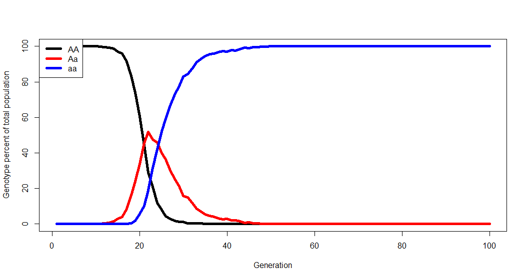
Chances are that whatever resultant dynamics you observe from the model have already been described by population geneticists. And that’s the point- you generate the biology, figure out what’s going on to lead you to the dynamics you observe, and learn how these biological phenomena have been previously described. There will also be a focus on the limitations of models and simulations.
Anyway, that’s my idea. Your thoughts are appreciated!
